Evaluation and statistics of expression data using NormalyzerDE
Jakob Willforss, Aakash Chawade and Fredrik Levander
02/03/2026
Source:vignettes/vignette.Rmd
vignette.RmdAbstract
Technical biases reduces the ability to see the desired biological changes when performing omics experiments. There are numerous normalization techniques available to counter the biases, but to find the optimal normalization is often a non-trivial task. Furthermore there are limited tools available to counter biases such as retention-time based biases caused by fluctuating electrospray intensities. NormalyzerDE helps this process by performing a wide range of normalization techniques including a general and openly available approach to countering retention-time based biases. More importantly it calculates and visualizes a number of performance measures to guide the users selection of normalization technique. Furthermore, NormalyzerDE provides means to easily perform differential expression statistics using either the empirical Bayes Limma approach or ANOVA. Evaluation visualizations are available for both normalization performance measures and as P-value histograms for the subsequent differential expression analysis comparisons. NormalyzerDE package version: 1.23.5
Installation
Installation is preferably performed using BiocManager (requires R version >= 3.5):
install.packages("BiocManager")
BiocManager::install("NormalyzerDE")
Default use
Input format
NormalyzerDE expects a raw data file. Columns can contain annotation information or sample data. Each column should start with a header.
pepseq  s1      s2      s3      s4
ATAAGG  20.0    21.2    19.4    18.5
AWAG    23.3    24.1    23.5    17.3
ACATGM  22.1    22.3    22.5    23.2
This data should be provided with a design matrix where all data samples should be represented. One column (default header “sample”) should match the columns containing samples in the raw data. Another column (default header “group”) should contain condition levels which could be used for group-based evaluations.
sample  group
s1      condA
s2      condA
s3      condB
s4      condB
Alternatively the data can be provided as an instance of a
SummarizedExperiment S4 class.
Running NormalyzerDE evaluation
The evaluation step can be performed with one command,
normalyzer. This command expects a path to the data file, a
name for the run-job, a path to a design matrix and finally a path to an
output directory.
Alternatively the designPath and dataPath
arguments can be replaced with the experimentObj argument
where the first assay should contain the data matrix of interest, the
colData attribute the design matrix and the
rowData attribute the annotation columns.
library(NormalyzerDE)
outDir <- tempdir()
designFp <- system.file(package="NormalyzerDE", "extdata", "tiny_design.tsv")
dataFp <- system.file(package="NormalyzerDE", "extdata", "tiny_data.tsv")
normalyzer(jobName="vignette_run", designPath=designFp, dataPath=dataFp,
           outputDir=outDir)
## You are running version 1.23.5 of NormalyzerDE## [Step 1/5] Load data and verify input## Input data checked. All fields are valid.## Sample check: More than one sample group found## Sample replication check: All samples have replicates## RT annotation column found (5)## [Step 1/5] Input verified, job directory prepared at:/tmp/RtmpVA6fHb/vignette_run## [Step 2/5] Performing normalizations## [Step 2/5] Done!## [Step 3/5] Generating evaluation measures...## [Step 3/5] Done!## [Step 4/5] Writing matrices to file## [Step 4/5] Matrices successfully written## [Step 5/5] Generating plots...## Warning: `aes_string()` was deprecated in ggplot2 3.0.0.
## ℹ Please use tidy evaluation idioms with `aes()`.
## ℹ See also `vignette("ggplot2-in-packages")` for more information.
## ℹ The deprecated feature was likely used in the vsn package.
## Please report the issue to the authors.
## This warning is displayed once per session.
## Call `lifecycle::last_lifecycle_warnings()` to see where this warning was
## generated.## [Step 5/5] Plots successfully generated## All done! Results are stored in: /tmp/RtmpVA6fHb/vignette_run, processing time was 0.2 minutesRunning NormalyzerDE statistical comparisons
When you after performing the evaluation and having evaluated the report have decided for which normalization approach seems to work best you can continue to the statistical step.
Here, expected parameters are the path to the target normalization matrix, the sample design matrix as in the previous step, a job name, the path to an output directory and a list of the pairwise comparisons for which you want to calculate contrasts. They are provided as a character vector with conditions to compare separated by a dash (“-”).
Similarly as for the normalization step the designPath
and dataPath arguments can be replaced with an instance of
SummarizedExperiment sent to the experimentObj
argument.
normMatrixPath <- paste(outDir, "vignette_run/CycLoess-normalized.txt", sep="/")
normalyzerDE("vignette_run",
             comparisons=c("4-5"),
             designPath=designFp,
             dataPath=normMatrixPath,
             outputDir=outDir,
             condCol="group")
## You are running version 1.23.5 of NormalyzerDE## [1] "Setting up statistics object"
## [1] "Calculating statistical contrasts..."
## [1] "Contrast calculations done!"
## [1] "Writing 100 annotated rows to /tmp/RtmpVA6fHb/vignette_run/vignette_run_stats.tsv"
## [1] "Writing statistics report"## [1] "All done! Results are stored in: /tmp/RtmpVA6fHb/vignette_run, processing time was 0 minutes"Running NormalyzerDE using a SummarizedExperiment object as input
A benefit of using a SummarizedExperiment object as input is that it allows executing NormalyzerDE using variables as input instead of loading from file.
The conversion of designMatrix$sample is required if
using read.table as it otherwise is interpreted as a
factor. For more intuitive behaviour you can use read_tsv
from the readr package instead of
read.table.
dataMatrix <- read.table(dataFp, sep="\t", header = TRUE)
designMatrix <- read.table(designFp, sep="\t", header = TRUE)
designMatrix$sample <- as.character(designMatrix$sample)
dataOnly <- dataMatrix[, designMatrix$sample]
annotOnly <- dataMatrix[, !(colnames(dataMatrix) %in% designMatrix$sample)]

sumExpObj <- SummarizedExperiment::SummarizedExperiment(
    as.matrix(dataOnly),
    colData=designMatrix,
    rowData=annotOnly
)

normalyzer(jobName="sumExpRun", experimentObj = sumExpObj, outputDir=outDir)
## You are running version 1.23.5 of NormalyzerDE## [Step 1/5] Load data and verify input## Input data checked. All fields are valid.## Sample check: More than one sample group found## Sample replication check: All samples have replicates## RT annotation column found (5)## [Step 1/5] Input verified, job directory prepared at:/tmp/RtmpVA6fHb/sumExpRun## [Step 2/5] Performing normalizations## [Step 2/5] Done!## [Step 3/5] Generating evaluation measures...## [Step 3/5] Done!## [Step 4/5] Writing matrices to file## [Step 4/5] Matrices successfully written## [Step 5/5] Generating plots...## [Step 5/5] Plots successfully generated## All done! Results are stored in: /tmp/RtmpVA6fHb/sumExpRun, processing time was 0.1 minutesRetention time normalization
Retention time based normalization can be performed with an arbitrary normalization matrix.
Basic usage
There are two points of access for the higher order normalization.
Either by calling getRTNormalizedMatrix which applies the
target normalization approach stepwise over the matrix based on
retention times, or by calling
getSmoothedRTNormalizedMatrix which generates multiple
layered matrices and combines them. To use them you need your raw data
loaded into a matrix, a list containing retention times and a
normalization matrix able to take a raw matrix and return a normalized
in similar format.
##      Cluster.ID Peptide.Sequence External.IDs Charge Average.RT Average.m.z
## 1 1493882053114       AAAAEINVKD       P38156      2   20.25051     501.268
##   s_12500amol_1 s_12500amol_2 s_12500amol_3 s_125amol_1 s_125amol_2 s_125amol_3
## 1     115597000     109302000     100314000    98182352    87241776    98702800
head(designDf, 1)## sample group batch
## 1 s_125amol_1 4 2At this point we have loaded the full data into dataframes. Next, we use the sample names present in the design matrix to extract sample columns from the raw data. Be careful that the sample names is a character vector. If it is a factor it will extract wrong columns.
Make sure that sample names extracted from design matrix are in right format. We expect it to be in ‘character’ format.
sampleNames <- as.character(designDf$sample)
typeof(sampleNames)
## [1] "character"Now we are ready to extract the data matrix from the full matrix. We also need to get the retention time column from the full matrix.
##      s_125amol_1 s_125amol_2 s_125amol_3 s_12500amol_1 s_12500amol_2
## [1,]    98182352    87241776    98702800     115597000     109302000
##      s_12500amol_3
## [1,]     100314000
If everything is fine the data matrix should be double,
and have the same number of rows as the number of retention time values
we have.
typeof(dataMat)## [1] "double"
print("Rows and columns of data")## [1] "Rows and columns of data"
dim(dataMat)## [1] 100 6
print("Number of retention times")## [1] "Number of retention times"
length(retentionTimes)## [1] 100The normalization function is expected to take a raw intensity matrix and return log transformed values. We borrow the wrapper function for Loess normalization from NormalyzerDE. It can be replaced with any custom function as long as the wrapper has the same input/output format.
performCyclicLoessNormalization <- function(rawMatrix) {
    log2Matrix <- log2(rawMatrix)
    normMatrix <- limma::normalizeCyclicLoess(log2Matrix, method="fast")
    colnames(normMatrix) <- colnames(rawMatrix)
    normMatrix
}
We are ready to perform the normalization.
rtNormMat <- getRTNormalizedMatrix(dataMat,
                                   retentionTimes,
                                   performCyclicLoessNormalization,
                                   stepSizeMinutes=1,
                                   windowMinCount=100)
Let’s double check the results. We expect a matrix in the same format and shape as before. Furthermore, we expect similar but not the exact same values as if we’d applied the normalization globally.
globalNormMat <- performCyclicLoessNormalization(dataMat)
dim(rtNormMat)
## [1] 100 6
dim(globalNormMat)## [1] 100 6
head(rtNormMat, 1)## s_125amol_1 s_125amol_2 s_125amol_3 s_12500amol_1 s_12500amol_2 s_12500amol_3
## 26.54027 26.36017 26.57715 26.7771 26.70227 26.59205
head(globalNormMat, 1)## s_125amol_1 s_125amol_2 s_125amol_3 s_12500amol_1 s_12500amol_2
## [1,] 26.54027 26.36017 26.57715 26.7771 26.70227
## s_12500amol_3
## [1,] 26.59205Performing layered normalization
We have everything set up to perform the layered normalization. The result here is expected to be overall similar to the normal retention time approach.
layeredRtNormMat <- getSmoothedRTNormalizedMatrix(
    dataMat,
    retentionTimes,
    performCyclicLoessNormalization,
    stepSizeMinutes=1,
    windowMinCount=100,
    windowShifts=3,
    mergeMethod="mean")

dim(layeredRtNormMat)
## [1] 100 6
head(layeredRtNormMat, 1)## s_125amol_1 s_125amol_2 s_125amol_3 s_12500amol_1 s_12500amol_2
## [1,] 26.54027 26.36017 26.57715 26.7771 26.70227
## s_12500amol_3
## [1,] 26.59205Stepwise processing (normalization part)
NormalyzerDE consists of a set of steps. The workflow can be run as a whole, or step by step.
Step 1: Loading data
This step performs input validation of the data, and generates an object of the class NormalyzerDataset.
jobName <- "vignette_run"
experimentObj <- setupRawDataObject(dataFp, designFp, "default", TRUE, "sample", "group")
normObj <- getVerifiedNormalyzerObject(jobName, experimentObj)
## Input data checked. All fields are valid.## Sample check: More than one sample group found## Sample replication check: All samples have replicates## RT annotation column found (5)The function setupRawDataObject returns a
SummarizedExperiment object. This object can be prepared
directly and should in that case contain the raw data as the default
assay, the design matrix as colData and annotation rows as
rowData.
Step 2: Generate normalizations
Here, normalizations are performed. This generates a NormalyzerResults object containing both a reference to its original dataset object, but also generated normalization matrices.
normResults <- normMethods(normObj)Step 3: Generate performance measures
Performance measures are calculated for normalizations. These are stored in an object NormalizationEvaluationResults. A NormalyzerResults object similar to the one sent in is returned, but with this field added.
normResultsWithEval <- analyzeNormalizations(normResults)Step 4: Output matrices to file
Generated normalization matrices are written to the provided folder.
jobDir <- setupJobDir("vignette_run", tempdir())
writeNormalizedDatasets(normResultsWithEval, jobDir)
Step 5: Generate evaluation plots
Performance measures are used to generate evaluation figures which is written in an evaluation report.
generatePlots(normResultsWithEval, jobDir)## agg_png
## 2After this evaluation of normalizations and progression to statistics follows as described previously in this report.
Stepwise processing (differential expression analysis part)
Step 1: Setup folders and data matrices
For continued processing you select the matrix containing the normalized data from the best performing normalization. The design matrix is the same as for the normalization step.
bestNormMatPath <- paste(jobDir, "RT-Loess-normalized.txt", sep="/")
experimentObj <- setupRawContrastObject(bestNormMatPath, designFp, "sample")
nst <- NormalyzerStatistics(experimentObj, logTrans=FALSE)
Similarly as to for the normalization evaluation step the
experimentObj above can be prepared directly as a
SummarizedExperiment object.
Step 2: Calculate statistics
Now we are ready to perform the contrasts. Contrasts are provided as
a vector in the format c("condA-condB", "condB-condC"),
where condX is the group levels.
comparisons <- c("4-5")
nst <- calculateContrasts(nst, comparisons, condCol="group", leastRepCount=2)
Step 3: Generate final matrix and output
Finally we generate a table containing the statistics results for each feature and write it to file together with an evaluation report containing P-value histograms for each comparison.
annotDf <- generateAnnotatedMatrix(nst)
utils::write.table(annotDf, file=paste(jobDir, "stat_table.tsv", sep="/"))
generateStatsReport(nst, "Vignette stats", jobDir)
## agg_png
## 2Code organization
NormalyzerDE consists of a number of scripts and classes. They are focused around two separate workflows. One is for normalizing and evaluating the normalizations. The second is for performing differential expression analysis. Classes are contained in scripts with the same name.
Code organization:
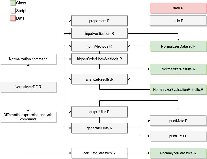
The standard workflow for the normalization is the following:
- The
normalyzerfunction in theNormalyzerDE.Rscript is called, starting the process. - If applicable (that is, input is in Proteois or MaxQuant format),
the dataset is preprocessed into the standard format using code in
preparsers.R. - The input is verified to capture standard errors early on using code
in
inputVerification.R. This results in an instance of theNormalyzerDatasetclass. - The data is normalized using several normalization methods present
in
normMethods.R. This yields an instance ofNormalyzerResultswhich links to the originalNormalyzerDatasetinstance and also contains all the resulting normalized datasets. - If specified (and if a column with retention time values is present)
retention-time segmented approaches are performed by applying
normalizations from
normMethods.Rover retention time using functions present inhigherOrderNormMethods.R. - The results are analyzed using functions present in
analyzeResults.R. This yields an instance ofNormalyzerEvaluationResultscontaining the evaluation results. This instance is attached to theNormalyzerResultsobject. - The final results are sent to
outputUtils.Rwhere the normalizations are written to an output directory, and togeneratePlots.Rwhich contains visualizations for the performance measures. It also uses code inprintMeta.RandprintPlots.Rto output the results in a desired format.
When a normalized matrix is selected the analysis proceeds to the statistical analysis.
- The
normalyzerdefunction in theNormalyzerDE.Rscript is called starting the differential expression analysis pipeline. - An instance of
NormalyzerStatisticsis prepared containing the input data. - Code in the
calculateStatistics.Rscript is used to calculate the statistical contrasts. The results are attached to theNormalyzerStatisticsobject. - The resulting statistics are used to generate a report and an annotated output matrix where key statistical measures are attached to the original matrix.
Used packages
## R version 4.5.2 (2025-10-31)
## Platform: x86_64-pc-linux-gnu
## Running under: Ubuntu 24.04.3 LTS
##
## Matrix products: default
## BLAS:   /usr/lib/x86_64-linux-gnu/openblas-pthread/libblas.so.3
## LAPACK: /usr/lib/x86_64-linux-gnu/openblas-pthread/libopenblasp-r0.3.26.so;  LAPACK version 3.12.0
##
## locale:
##  [1] LC_CTYPE=C.UTF-8       LC_NUMERIC=C           LC_TIME=C.UTF-8
##  [4] LC_COLLATE=C.UTF-8     LC_MONETARY=C.UTF-8    LC_MESSAGES=C.UTF-8
##  [7] LC_PAPER=C.UTF-8       LC_NAME=C              LC_ADDRESS=C
## [10] LC_TELEPHONE=C         LC_MEASUREMENT=C.UTF-8 LC_IDENTIFICATION=C
##
## time zone: UTC
## tzcode source: system (glibc)
##
## attached base packages:
## [1] stats     graphics  grDevices utils     datasets  methods   base
##
## other attached packages:
## [1] NormalyzerDE_1.23.5
##
## loaded via a namespace (and not attached):
##  [1] SummarizedExperiment_1.40.0 gtable_0.3.6
##  [3] xfun_0.56                   bslib_0.10.0
##  [5] ggplot2_4.0.1               Biobase_2.70.0
##  [7] lattice_0.22-7              vctrs_0.7.1
##  [9] tools_4.5.2                 generics_0.1.4
## [11] parallel_4.5.2              stats4_4.5.2
## [13] tibble_3.3.1                vsn_3.78.1
## [15] pkgconfig_2.0.3             Matrix_1.7-4
## [17] RColorBrewer_1.1-3          S7_0.2.1
## [19] desc_1.4.3                  S4Vectors_0.48.0
## [21] lifecycle_1.0.5             compiler_4.5.2
## [23] farver_2.1.2                textshaping_1.0.4
## [25] statmod_1.5.1               Seqinfo_1.0.0
## [27] carData_3.0-6               htmltools_0.5.9
## [29] sass_0.4.10                 yaml_2.3.12
## [31] preprocessCore_1.72.0       Formula_1.2-5
## [33] hexbin_1.28.5               pkgdown_2.2.0
## [35] pillar_1.11.1               car_3.1-3
## [37] jquerylib_0.1.4             MASS_7.3-65
## [39] affy_1.88.0                 DelayedArray_0.36.0
## [41] cachem_1.1.0                limma_3.66.0
## [43] abind_1.4-8                 nlme_3.1-168
## [45] tidyselect_1.2.1            digest_0.6.39
## [47] dplyr_1.1.4                 labeling_0.4.3
## [49] splines_4.5.2               fastmap_1.2.0
## [51] grid_4.5.2                  cli_3.6.5
## [53] SparseArray_1.10.8          magrittr_2.0.4
## [55] S4Arrays_1.10.1             ape_5.8-1
## [57] withr_3.0.2                 scales_1.4.0
## [59] rmarkdown_2.30              XVector_0.50.0
## [61] affyio_1.80.0               matrixStats_1.5.0
## [63] ragg_1.5.0                  evaluate_1.0.5
## [65] knitr_1.51                  GenomicRanges_1.62.1
## [67] IRanges_2.44.0              mgcv_1.9-3
## [69] rlang_1.1.7                 Rcpp_1.1.1
## [71] glue_1.8.0                  BiocManager_1.30.27
## [73] BiocGenerics_0.56.0         jsonlite_2.0.0
## [75] R6_2.6.1                    MatrixGenerics_1.22.0
## [77] systemfonts_1.3.1           fs_1.6.6